I was recently given the task of finding the best location for a company's office. The company, located in central London, had about 100 people and needed to move out of their current office. Even before doing any spatial analysis, it seems intuitive to think that the current distribution of employees' residence was informed by the location of the office, and therefore the best office location would be central London. But how different would be the impact if the office was moved East London, or West London? Performing a spatial analysis to understand the impact of this change on people's transport journey is therefore primordial for any company that pretend to attract innovation and talent - these employees can, and will, change of company if their commute suddenly becomes to much of a pain.

I conducted three analyses:

• Assessment of the current situation: how long does it take employee's to travel
• Finding the hot and cold spots of office locations (most people better off/worth off)
• Comparing potential office locations

Data

Employee data

I was given the postcode of each employee (in the UK, a postcode is usually given to 10-20 addresses, so using the postcode is a good enough approximation to people's location). I first needed to locate them in terms of geographic coordinates. There are at least two free ways to do this: either you happen to already have the data with the geographic coordinates for each postcode (the data is currently sold I believe by the PostOffice, but there are outdated versions on the web), or you use a geolocating service (e.g. google maps API). If you have a small number of addresses and not much budget, the best is probably to use a free geolocation service such as the google maps API.

I used google maps geolocating service: there are some QGIS plugins that use it, or a python google maps API wrapper library. I used QGIS, but if you wanted to use the python library, then you should register an API key (there is a key per service) and use the code below:

import google maps
gmaps = google maps.Client(key='YOUR API KEY HERE')
lpostcodes = ['W1N 4AD', 'NB6 9UI']
# Geocoding an address
# geocode_result = gmaps.geocode('1600 Amphitheatre Parkway, Mountain View, CA')
lcoords = []
for pc in lpostcodes:
    geocode_result = gmaps.geocode(pc)
    l.coords.append(geocode_result)

Transit data

At first I downloaded the TfL station data, which contains all the TFL (tube and overground) stations and the lines that are deserved there. I used the QGIS analysis called Distance matrix, roughly following these steps. It gave me the three or more closest stations and I was also able to find the list of most accessible lines to all employees. Although this was interesting to find out, practically I wasn't much closer to finding a potential office location without including real transport data. Also, the TFL data excluded some train stations, which made the analysis obviously flawed.

I knew the best analysis would be a network analysis, which would include real public transport data, but this was meant to be low-key analysis, not full-on spatial analysis. Seriously, is there any company out there that would give the transport time for any journey and would include any means of transport? Well, obviously there is google maps! Google gives a restricted access for free to its direction API. The restrictions boil down to 2,500 API calls per day (and less than 100 per call). With about 100 employees, that's easily done!

Another option would have been to use the TfL API, but I think it would include less options that google maps.

I registered a key with the Google services for the direction API.

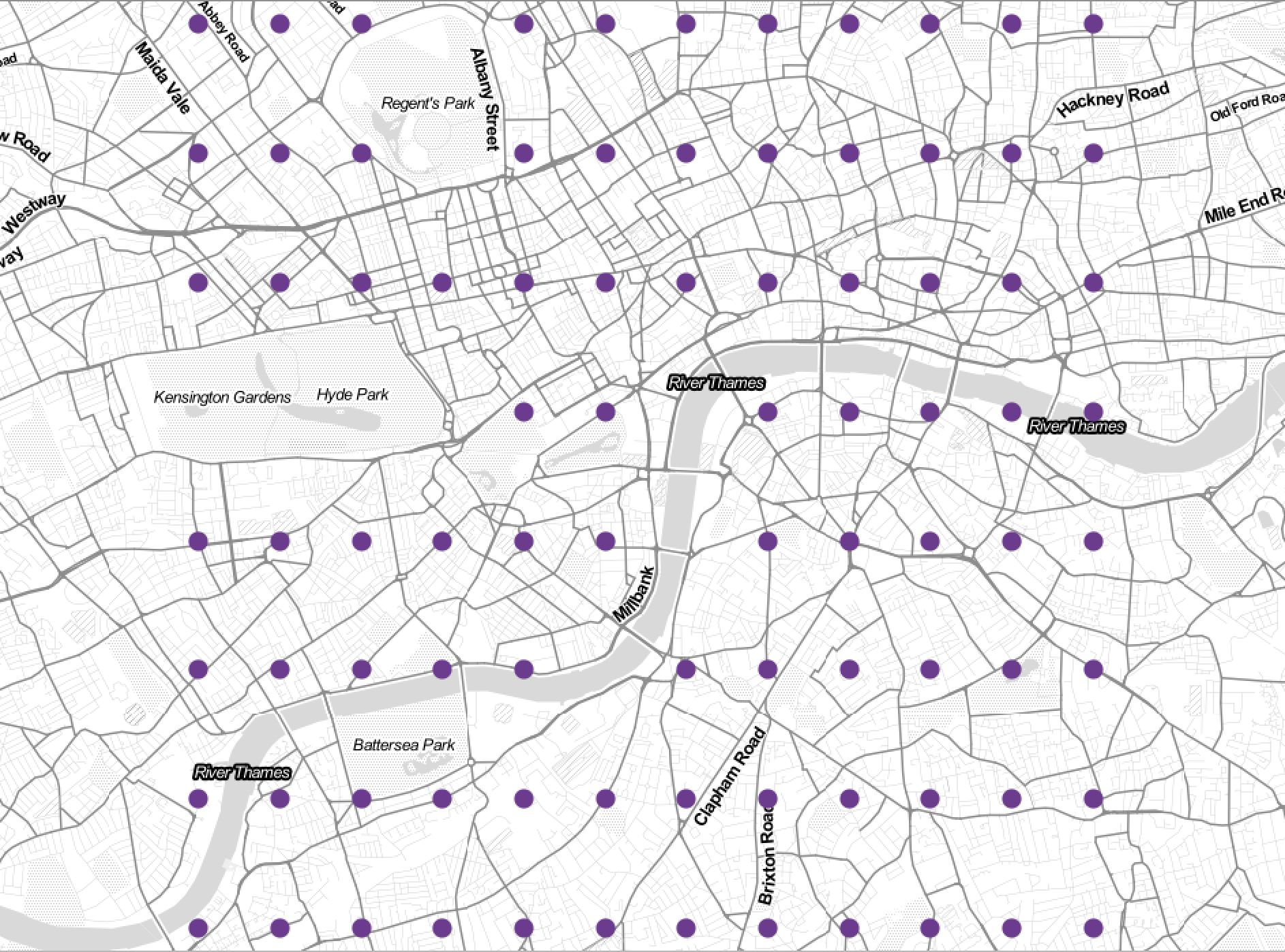
Making a grid

To find hot and cold spots of office location, I needed a grid of points equally spaced and for which I would calculate the travel time for each employee. I used python to create such a grid, using a meshgrid inside a rectangle for which I defined the min/max of X. I found this with google maps, to cover central London, and used a 0.01 deg step.

## Generate a grid with points around the current office
## Based on https://stackoverflow.com/questions/35418012/how-to-create-matrix-of-points-by-x-y-coordinate-in-python
import numpy as np
import csv

# define the lower and upper limits for x and y
minX, maxX, minY, maxY = -0.224155, 0.042997, 51.464841, 51.536015
# create one-dimensional arrays for x and y
x = np.linspace(minX, maxX, (maxX-minX)/0.01+1)
y = np.linspace(minY, maxY, (maxY-minY)/0.01+1)
# create the mesh based on these arrays
X, Y = np.meshgrid(x, y)
# .. or as tuples
coords = zip(X, Y)

with open('meshgrid_officelocations.csv','w') as f:
    writer = csv.writer(f)
    writer.writerow(["placeid","y","x"])
    for x,y in coords:
        for i in range(len(x)):
            writer.writerow([i,x[i],y[i]])

Rent price data

I was curious to find the impact of the office rental price on employees transit duration. Would the rental price be higher or lower in each hot and cold spot? I used the rental office price tube map made by Thrisllist. There were 69 stations in Zone 1, with a monthly individual price from £450 in Lancaster Gate to £1,000 in Paddington, South Kensington, and St. James's Park.

Analysis

I present here three of the analyses I made for this question.

Question 1: Current situation

I used the Google Maps direction API to calculate the time for each employee to reach the office. Since officially work starts at 9.30am, I based my calculation for an arrival at 9.30am. The answer from the API is a nested json string containing all the information displayed on the Google Maps direction webpage: the time of departure and arrival, the duration, name of transport and company, changes, and every step of the journey. It also contains more than one option, the first being the fastest. Caveats are that it doesn't give the price, and in London that can be quite significant: buses are cheaper than the tube, which is cheaper than the DLSR. Not sure where the overground and the regional trains sit here.

I first prepared the date dynamically (to be able to run any day without hardcoding it!). :::python from datetime import datetime, timedelta now = datetime.now() tomorrow_morning = None if now.hour < 6: tomorrow_morning = datetime(now.year, now.month, now.day, 9, 30, 0, 0) else: tomorrow = datetime.today() + timedelta(days=1) tomorrow_morning = datetime(tomorrow.year, tomorrow.month, tomorrow.day, 9, 30, 0, 0) print(tomorrow_morning)

The transit time from the google maps direction API is given in two formats: machine readable (in second), and human readable (a nice string x hours y minutes). You can access it as follow:

import gmaps
dir_res = gmaps.directions(departure,destination,mode="transit",arrival_time=tomorrow_morning)
time_text = dir_res[0]['legs'][0]['duration']['text']
time_s = dir_res[0]['legs'][0]['duration']['value']

The Direction API sometimes fails, when it cannot find any transit option, so I added a check that there was an answer, and looped through the employees locations to find the time for every employee.

# Employee location
employee_pc = []
with open("employee_pc.csv",'r') as f:
    reader = csv.reader(f)
    for row in reader:
        employee_pc.append([row[0],row[1]])

transit_time = []
destination = 'Address of the office'
for pc in employee_pc:
        dir_res = gmaps.directions(pc[1],destination,mode="transit",departure_time=tomorrow_morning)
        if len(dir_res) != 0:
                transit_time.append([pc[0],pc[1],dir_res[0]['legs'][0]['duration']['text'],dir_res[0]['legs'][0]['duration']['value']])
        else:
                transit_time.append([pc[0],pc[1],np.nan,np.nan])

transit_time is a list of list, which is easy to write into a pandas dataframe. I quickly realised that some people in this company were living far away and therefore unlikely to go to the office every day.

import pandas as pd

headings = ['employeeid','postcode','duration','duration_s']
# Make a dataframe
df = pd.DataFrame(transit_time,columns=headings)

# Basic statistics
mean_dur = df['duration_s'].mean()/60
median_dur = df['duration_s'].median()/60

# This includes everyone, including those who don't go to the office every day.
# We can restrict to those who travel less than 1h30
df_short = df.copy()
df_short = df_short[df_short['duration_s']<5388]

mean_short_dur = df_short['duration_s'].mean()/60
median_short_dur = df_short['duration_s'].median()/60

# Categorise
df.ix[df['duration_s']<1800,'cat'] = 'Less than 0.5 hour'
df.ix[(df['duration_s']>1800) & (df['duration_s']<3600),'cat'] = 'Less than 1 hour'
df.ix[df['duration_s']>3600,'cat'] = 'More than 1 hour'

nb_lessthan05h = len(df[df['cat'] == 'Less than 0.5 hour'])
nb_lessthan1h = len(df[df['cat'] == 'Less than 1 hour'])
nb_morethan1h = len(df[df['cat'] == 'More than 1 hour'])

Question 2: Hot and Cold spot of office locations

In the second analysis I looked for hot and clod spots for office location. This is probably the most in-depth spatial analysis of this post. Instead of looking at current status or scenarios, it models London with an equidistant grid and systematically calculate the duration of each employee to each location.

That's when I actually hit the restrictions of the API, since with about 100 employees, the restriction is reached with 25 locations; while London was modeled with 87 points. I selected zone 1, corresponding to 28 points, and ran the analysis on two separate days.

API calls to calculate transit time for each employee to the every point of the grid

# List of destinations
XYnewoffices = []
with open('offices.csv','r') as f:
        reader = csv.reader(f)
        next(reader, None)
        for row in reader:
                XYnewoffices.append([row[0],str(row[1])])
# list of staff locations
staffloc = []
with open('staff.csv','r') as f:
        reader = csv.reader(f)
        next(reader, None)
        for row in reader:
                staffloc.append([row[2],row[8]])
dur_arr = []
i=0
dur_arr.append(["placeid","X","Y","employee_id","staff_postcode","duration","duration_s"])
for xy in XYnewoffices:
        dest_new = ",".join([str(xy[1]),str(xy[0])])
        i += 1
        for staff in staffloc:
                dir_res = gmaps.directions(staff[1],dest_new,mode="transit",departure_time=tomorrow_morning)
                if len(dir_res) != 0:
                        dur_arr.append([i,xy[0],xy[1],staff[0],staff[1],dir_res[0]['legs'][0]['duration']['text'],dir_res[0]['legs'][0]['duration']['value']])
                else:
                        dur_arr.append([i,xy[0],xy[1],staff[0],staff[1],np.nan,np.nan])

headers = ["placeid","X","Y","employee_id","staff_postcode","duration","duration_s"]
df = pd.DataFrame()

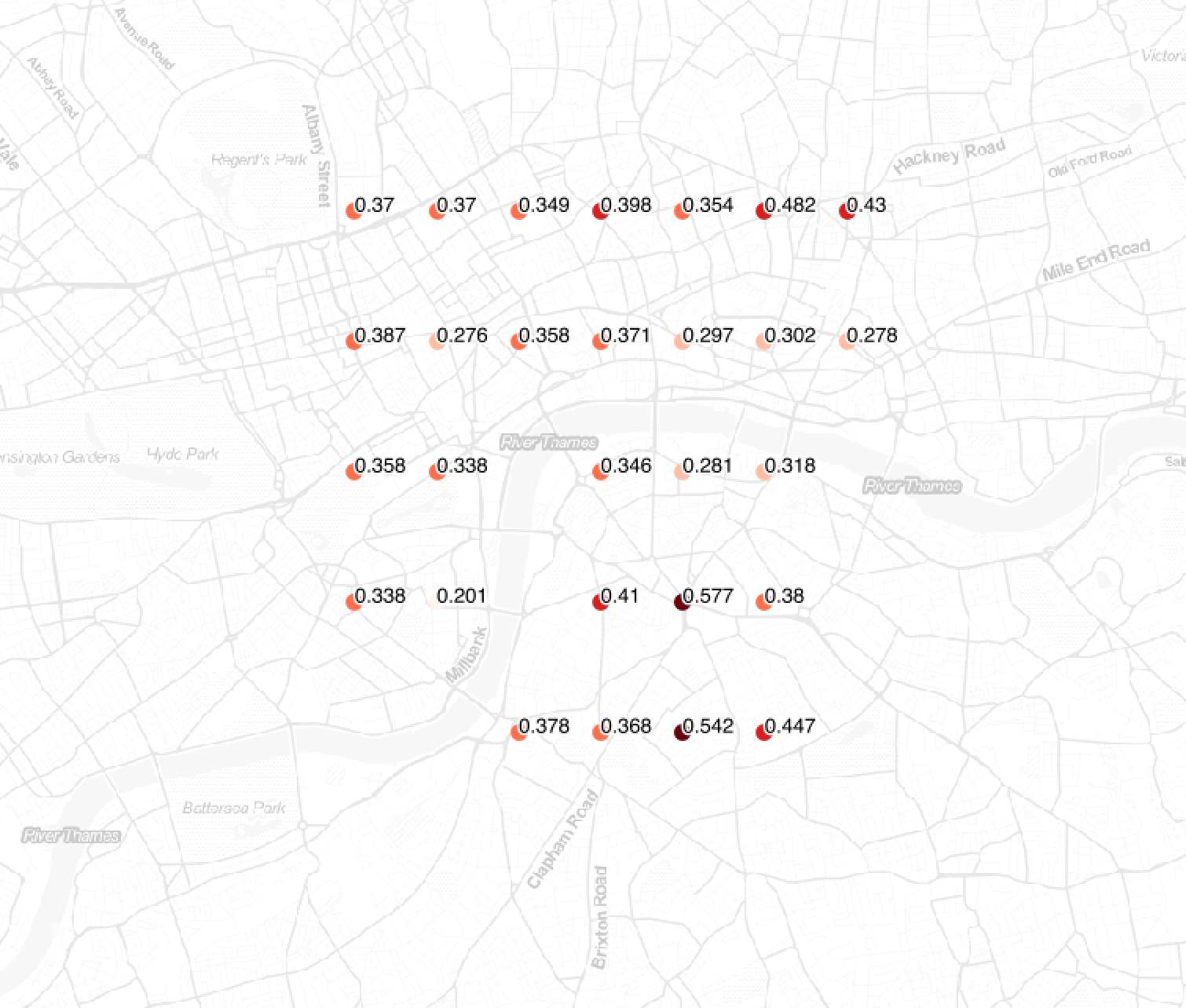
I exported this data to a CSV and imported it in QGIS. A simple chloropeth map highlights the places in London which are easier or more difficult to reach by the staff.

On its own, it's an interesting result, because if you're interested in your staff's commuting time, this narrows down quickly which places can be investigated or which one should be avoided.

Adding rental price

I also wanted to find the rental price for each point on that grid. I calculated the Voronoi polygons around the 59 tube stations: the borders of these polygons are equidistant of the closest two points; and therefore any point in a polygon is closer to the centre of that polygon, and so is given the its characteristics. A spatial join between the Voronoi polygons and the grid links the rental of price of the closest tube station to the grid.

I exported this data to csv again to import in python.

import pandas as pd

# Find the average time spent in transit per location
df['av_dur'] = df.groupby(['placeid'])['duration_s'].transform('mean')

# Divide in three groups based on their transit time:
# * Less than 30 minutes
# * 30 min to 1 hour
# * More than 1 hour
df.ix[df['duration_s']<1800, 'duration_group'] = 'lessthan30min'
df.ix[(df['duration_s']>1800)&(df['duration_s']<3600), 'duration_group'] = '30minto1hour'
df.ix[df['duration_s']>3600, 'duration_group'] = 'morethan1hour'

# Create a pivot table to count the number of employees in each group for each location
table = pd.pivot_table(df,values='employee_id',index=['placeid'],columns = 'duration_group', aggfunc = 'count')
table = table.reset_index()

# Merge the transit time for each location to the pivot table in order
# This creates a summary for each location
df_summary = df.merge(table,on='placeid')
df_summary = df[['placeid','lessthan30min','30minto1hour','morethan1hour','RentalPrice']]
df_summary = df_summary.drop_duplicates(['placeid'])

# Calculate a few scores based on the number of people contained in each of the three transit time groups:
# The higher the score, the better: people with a shorter commute weigh more than those with a longer commute
df_summary['score'] = 5*df['lessthan30min'] + 3*df['30minto1hour'] + 1*df['morethan1hour']
df_summary['score2'] = 10*df['lessthan30min'] + 5*df['30minto1hour'] + 1*df['morethan1hour']
df_summary['score3'] = 5*df['lessthan30min'] + 3*df['30minto1hour']

# The score is divided by the rental price, so the higher the rental price, the smaller the index is.
df_summary['scorePrice'] = df_summary['score']/df_summary['Price']

We obtain a map with a scorePrice index, which is higher when more employees travel less and the price is lower. We obtain the following map.

Comparison of potential office locations

Eventually, the company narrowed down to four choices for their new office locations. They wanted to understand the impact for all employees, as well as understanding who would be affected the most for each location (for employees not coming every day, then the impact would be lower overall).

They gave me a list of four postcodes, which I processed with Google Maps Direction API. :::python import csv import google maps from datetime import datetime, timedelta import pandas as pd, numpy as np

gmaps = google maps.Client(key='HERE YOUR API KEY')

# Prepare date
now = datetime.now()
tomorrow_morning = None

if now.hour < 6:
    tomorrow_morning = datetime(now.year, now.month, now.day, 9, 30, 0, 0)
else:
    tomorrow = datetime.today() + timedelta(days=1)
    tomorrow_morning = datetime(tomorrow.year, tomorrow.month, tomorrow.day, 9, 30, 0, 0)


# List of destinations: placeid, postcode
XYnewoffices = []
with open("4officelocations.csv",'r') as f:
    reader = csv.reader(f)
    next(reader, None)
    for row in reader:
        XYnewoffices.append([row[0],row[1]])


# list of staff locations: employee_id, postcode
staffloc = []
with open("../staff_loconly.csv",'r') as f:
    reader = csv.reader(f)
    next(reader, None)
    for row in reader:
        staffloc.append([row[0],row[6]])

# Loop through both lists and call API
time_arr = []
for staff in staffloc:
    print 'staff', staff[0], staff[1]
    stafftime = []
    stafftime.extend([staff[0], staff[1]])
    for i in range(len(XYnewoffices)):
        dir_res = gmaps.directions(staff[1],XYnewoffices[i][1],mode="transit",departure_time=tomorrow_morning)
        if len(dir_res) != 0:
            stafftime.extend([dir_res[0]['legs'][0]['duration']['text'],dir_res[0]['legs'][0]['duration']['value']])
        else:
            stafftime.extend([np.nan,np.nan])
    time_arr.append(stafftime)

# Make a pandas dataframe
headers = ["employee_id","employee_address",\
                 "Current_time","Current_time_s",\
                 "Option1_time","Option1_time_s",\
                 "Option2_time","Option2_time_s",\
                 "Option3_time","Option3_time_s",\
                 "Option4_time","Option4_time_s"]
df = pd.DataFrame(time_arr,columns=headers)

# Calculate gain and loss for each location for each employee
df['Option1_change'] = df['Option1_time_s'] - df['Current_time_s']
df['Option2_change'] = df['Option2_time_s'] - df['Current_time_s']
df['Option3_change'] = df['Option3_time_s'] - df['Current_time_s']
df['Option4_change'] = df['Option4_time_s'] - df['Current_time_s']


df_comp = df.copy()
df_comp = df_comp[['employee_id','Option1_change','Option2_change','Option3_change','Option4_change']]


# For each option, calculate:
 # the number of people for whom it is worse,
 # the average change for those negatively affected,
 # median for those negatively affected

# Melt the four option columns
df_melt = pd.melt(df_comp,value_vars=['Option1_change','Option2_change','Option3_change','Option4_change'])#id_vars=,

# Calcualte median: half employees are below this threshold, half are above.
df_median = df_melt.copy()
df_median = df_median.groupby(['variable']).agg({'value':np.median})
df_median = df_median.reset_index()
df_median = df_median.rename(columns={'variable':'option','value':'median'})
df_mean = df_melt.copy()
# Only calculate mean on the positive change values (for those that were affected negatively)
df_mean = df_mean.groupby(['variable']).agg(lambda x:x[x>0].mean())   
df_mean = df_mean.reset_index()
df_mean = df_mean.rename(columns={'variable':'option','value':'mean'})

# Merge
df_summary = df_median.merge(df_mean,on='option')

When trying to minimalise the impact of moving the office on employees' travelling time, we want to look at the difference of commuting time for each employee, rather than the new commuting time.

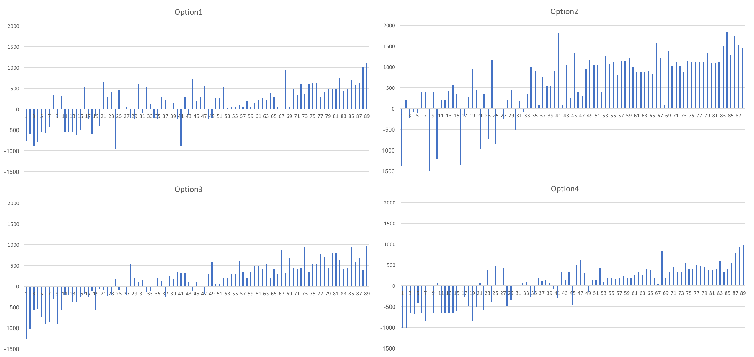
I first compared the number of people negatively affected (increase of commuting time), the average, max and median change of time (in minutes) for each option.

Nb people <0    Average (min.)  Max (min.)  Median (min.)

Option1 58 389.9482759 1101 205 Option2 74 878.0945946 2025 880 Option3 58 407.7413793 977 208 Option4 60 320.4666667 980 157

This clearly eliminate Option2: it's really the furthest away, and will increase commuting time for nearly all employees.

I also quickly produced graphs with the amount of time increased of decreased from commuting time for each employee.

Conclusion

This king of questions are really interesting, and I'm glad that companies care enough about their employees to seek information where it can help them making better decisions!